Introduction to Cable

Introduction to Cable_Two

Common advanced problems with high-frequency cables

Common advanced problems with high current cables

With basic knowledge, one can usually know "how to choose which cable". However, in practical applications, the problem is usually not "choosing the wrong cable", but rather misjudging a certain physical characteristic, such as:

Impedance discontinuities causing reflection and eye-diagram collapse

Thermal model misses by 30%, cable dies in a third of its rated life

Loss growing non-linearly with frequency — fine at 28 G, broken at 56 G

Cables bundled in trays, ampacity halves versus the table

Connectors hitting unexpected resonant modes past 50 GHz

Short-circuit event burns through insulation in seconds

NRZ hitting the wall, forcing a redesign around PAM4 equalization

Water treeing takes out XLPE underground cable after 20 years

00 / Discussion on the advanced application of high-frequency cable and high-current cable

01 / High-Frequency Advanced From "cable" to "transmission line"

High-frequency cables are often discussed for their characteristic impedance, which is often described as "50Ω or 100Ω". But how exactly is this number calculated? What happens when it's mismatched?

1.1 Transmission Line Theory: Treat the Cable as a Waveguide

When the signal wavelength approaches the physical length of the cable, voltage and current are no longer scalars — they propagate as travelling waves.

The cable must then be modelled as a distributed parameter network: per unit length, it has L (inductance), C (capacitance), R (resistance) and G (leakage conductance).

(a)Characteristic impedance(Z₀): Z₀=√( (R + jωL) / (G + jωC) ) ≈ √( L / C )（high-frequency, low-loss approximation）

Characteristic impedance is an intrinsic cable property, independent of length. For a coax: Z₀ = (60/√εᵣ) · ln(b/a), where a is the center-conductor radius, b is the inner shield radius, εᵣ is the relative permittivity.

(b)Reflection Coefficient (Γ): when the line ends in a mismatched load, part of the energy reflects back to the source.

Γ=(ZL− Z₀) / (ZL+ Z₀)

Γ = 0 means perfect match; Γ = ±1 means total reflection (open or short). Return loss RL = −20 log|Γ|. VSWR = (1+|Γ|)/(1−|Γ|).

(c)Standing-wave illustration:When wavelength is comparable to cable length, mismatched reflections create standing waves: voltage maxima and minima along the line.

The longer the cable and the higher the frequency, the worse the effect.

1.2 Loss Mechanisms: Why High-Frequency Signals Fade

How much does the signal attenuate per metre (dB/m)? That number grows non-linearly with frequency, driven by three overlapping loss mechanisms:

① Conductor loss α_c Caused by the skin effect. Current flows only on the surface; frequency ↑ → effective cross-section ↓ → resistance ↑.

α_c ∝ √f · Rs / (2π · a · ln(b/a))(coax, where Rs is surface resistivity)

② Dielectric loss α_d Dielectric molecules repeatedly polarize in the alternating field, dissipating heat.

α_d ∝ f · √εᵣ · tan δ(tan δ = loss tangent, the key material figure of merit)

③ Proximity effect Current crowding between adjacent conductors raises effective AC resistance. Especially severe in twisted pairs and dense differential pairs.

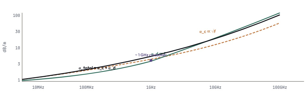
Typical coax total loss vs frequency

Below ~1 GHz conductor loss dominates; above it, dielectric loss takes over. That's why mmWave cables chase ultra-low-Df materials (foam PE, PTFE).

1.3 S-Parameters & TDR: The Language of Measurement

S-parameters (Scattering Parameters)describe how a two-port network reflects and transmits at a given frequency:

Parameter	Meaning	Ideal
S11	Port-1 reflection coefficient (dB)	−∞ (lower better)
S21	Port-1 → 2 transmission (dB)	0 (lower better)
S12	Port-2 → 1 isolation (dB)	−∞ (reverse isolation)
S22	Port-2 reflection coefficient (dB)	−∞

The frequency where S21 = −3 dB defines the cable's−3 dB bandwidth— the half-power point.

TDR (Time Domain Reflectometry): send a fast pulse down the line, look at the reflection's timing and amplitude — you can locateimpedance discontinuitiesand tell whether they're open, short, or somewhere in between.

Positive reflection = open or high-Z; negative reflection = short or low-Z. Time-axis × propagation velocity = fault location.

1.4 Dielectric Materials: Dk and Df Are What Matter

Two numbers decide high-frequency performance: Dk = εᵣ(permittivity, sets impedance and propagation velocity) and Df = tan δ(loss tangent; the lower the better).

The table shows typical values at 1-10 GHz.

Material	Dk (εᵣ)	Df (×10⁻⁴)	Temp °C	Typical Use
Solid PE	2.3	2-4	75	RG58 / RG174, low-loss RF cables
Foam PE	1.4-1.6	1-3	85	CATV distribution, semi-rigid jumpers
PTFE (Teflon)	2.1	2-4	260	Semi-rigid, mmWave, aerospace
FEP	2.1	5-7	200	High-temp RF cables (RG316)
Air (helical spacer)	~1.1	<1	—	HELIAX, broadcast feeders, lowest loss
LCP (Liquid Crystal Polymer)	2.9-3.2	2-4	270	5G flex circuits, USB4 flex substrates

Semi-rigid cables use solid PTFE for minimum loss but cannot be re-bent; flexible coax uses foam PE as a compromise.

1.5 Coaxial Connector Frequency Limits

A connector's max usable frequency is set by the size of its internal air-dielectric section— when the signal wavelength approaches that opening, unwanted propagation modes (TE11) get excited.

The industry response has been a steady shrinking of that air gap:

1.6 High-Speed Signaling Evolution: NRZ → PAM4 → 224G

The signal rate has roughly doubled every generation for 30 years. Around 56 Gbps NRZ the channel hit a physical wall, and the industry shifted to PAM4 (4-level pulse-amplitude modulation) — 2 bits per symbol in exchange for half the Nyquist bandwidth.

Channel-loss budget evolution

Generation	Modulation	Nyquist loss budget
10G KR	NRZ	~ 8 dB @ 5 GHz
25G KR	NRZ	~ 10 dB @ 12.5 GHz
56G PAM4	PAM4	~ 13 dB @ 14 GHz
112G PAM4	PAM4	~ 16 dB @ 28 GHz
224G PAM4	PAM4	~ 20 dB @ 56 GHz

Key interface standards

PCIe Gen5/6: 32 / 64 GT/s PAM4, intra-server

USB4 v2: 80 Gbps PAM3 + dual-lane

HDMI 2.1: 48 Gbps, fixed-cable architecture

IEEE 802.3ck: 100G / 200G / 400G Ethernet

OIF CEI-224G: next-generation chip-to-chip

Loss budget=ILcable+ ILconnector+ ILpcb+ ILcrosstalk≤TX EQ headroom + RX EQ headroom

Sum of every component's loss must fit inside the combined equalization headroom of Tx and Rx. Cross the line and BER collapses.

1.7 Equalization: When the Channel Runs Out

By 112G, "just buy a better cable" no longer scales fast enough. The industry reaches for three equalizers to claw back the high-frequency loss:

(a)CTLE: Continuous Time Linear EQ.

A high-pass filter at the receiver that "lifts" the high frequencies, compensating channel roll-off. Passive, simple, low power.

(b)FFE: Feed-Forward EQ.

At the transmitter, sum multiple delayed, weighted copies of the signal (pre-emphasis / de-emphasis) to pre-compensate the channel.

(c)DFE: Decision Feedback EQ.

At the receiver, subtract ISI using already-decided bits. Most powerful, but adds latency and power.

In practice a 112G SerDes usually runs CTLE + DFEat Rx and adds FFE at Tx. The combined goal: open the eye.

02 / High-Current Advanced From "AWG chose" to "Life consideration"

Many people choose cable by looking up ampacity in a table. But,where did the table come from, how does your real installation differ, and what happens at end of life?

2.1 Heat Balance: The Real Meaning Behind Ampacity

Ampacity is not "thicker copper = more current, period". It's a thermal equilibrium: the Joule heat generated in the conductor must equal the heat shed from the insulation surface to the surroundings.

(a)Form: I² · Rac=(Tc− Ta) / (Rth,dielectric+ Rth,jacket+ Rth,ambient)

T_c = conductor operating temperature, T_a = ambient temperature, R_th = thermal resistance of each layer, R_ac = AC resistance (includes skin and proximity effects).

(b)Simplified form (single-core, free air)

I=√[ (Tc− Ta) · h · π · d / Rac]

h is the surface heat-transfer coefficient (W/m²·K), d is the conductor outer diameter. For small cables h is roughly 5-15 W/m²·K in free air.

(c)Buried cables (IEC 60287)

Adds soil thermal resistivity(typically 1.0-2.5 K·m/W), burial depth, and thermal coupling to neighbouring cables. IEC 60287 is a full set of iterative formulas that handle multi-core, armoured, HDPE-jacketed constructions.

(d)The Neher-McGrath method(the empirical approach used by NEC) reduces the above heat balance to a lookup-table-friendly approximation. It is within ±5% for 600 V cables, but for high-voltage (≥ 5 kV) or non-standard installations you still need the full IEC 60287 treatment.

2.2 Derating Factors: Why the Table Number Always Gets Discounted

The table assumes a reference condition— usually 30°C ambient, single conductor, in free air. Real installations layer multiple derating factors on top:

Ambient temperature (NEC Table 310.15(B)(1))

Ambient °C	90°C rated	75°C rated
30	1	1
40	0.91	0.88
50	0.82	0.75
60	0.71	0.58
70	0.58	—

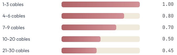
Bundling (NEC Table 310.15(C)(1))

2.3 Voltage Drop: Different Circuits, Different Formulas

(a)DC:Vdrop=2 · I · R · L（out and back）

(b)Single-phase AC:Vdrop=2 · I · L · (R cosφ + X sinφ)（X is the reactance, can't be ignored for large cables）

(c)Three-phase AC:Vdrop=√3 · I · L · (R cosφ + X sinφ)（most industrial distribution）

Practical rule of thumb:low-voltage distribution (≤ 1000 V) usually requires voltage drop≤ 3%(lighting) or≤ 5%(power); from the transformer to the most distant load, total drop must not exceed 5%(NEC 210.19 / 215.2).

The cos φ effect:for a pure resistive load cos φ = 1 and the formula collapses to 2·I·R·L. For inductive loads (motors) cos φ = 0.7-0.85, and the reactance X matters — typically 0.07-0.1 Ω/km for cables ≥ 35 mm².

2.4 Short-Circuit Withstand: Can the Insulation Hold?

During a short circuit, the current can spike to10-30× normal for 0.1-5 seconds. In that brief window the conductor has no time to shed heat — all the energy goes into heating up the copper and the insulation.The insulation must survive that temperature spike without breaking down.

Amin=Isc· √t / k

A_min = minimum allowable cross-section (mm²), I_sc = short-circuit current (A), t = protection time (s), k = material constant.

k examples: PVC 115, XLPE 143, EPR 141. XLPE's higher thermal tolerance lets you use a smaller cross-section for the same fault current.

In practice:the I²t method is most common. The breaker's time-current curve must sit below and to the left of the cable's I²t-withstand curve to provide protection.

2.5 Insulation Aging: The Cable's "Lifetime Equation"

Insulation polymers degrade over time. The Montsinger rule("10°C rule") says: every 10°C above rated temperature, life halves.

(a)The Arrhenius equation is used:

L(t)=L₀ · exp[ (Ea/ k) · (1/T − 1/T₀) ]

E_a = activation energy (PVC ~80 kJ/mol, XLPE ~110 kJ/mol), T is absolute temperature (K).

At the same operating temperature, XLPE lasts roughly 5-10× longer than PVC.

(b)Common aging phenomena

(b-1)Thermal aging

Long-term heat breaks polymer chains. PVC at 60°C ≈ 30 years; at 80°C ≈ 7-8 years.

(b-2)Water treeing

XLPE underground cables under water + electric field grow tree-like micro-channels inside the insulation; breakdown after 20-30 years.

(b-3)Electrical treeing

MV/HV cables develop branch-like damage at partial-discharge sites. Detectable early with a PD detector.

2.6 Specialized Applications: HVDC, 800V EV, Submarine

(a)HVDC

Up to ±525 kV at 2000 MW class. XLPE is replacing traditional oil-impregnated paper insulation for lower loss and zero maintenance. China's Baihetan–Jiangsu link is built on domestic 535 kV XLPE DC cable.

(b)800V EV architecture

Versus 400 V systems, 800 V halves the current for the same power— smaller cables, lower loss. The challenge is the high-frequency switching(PWM edges with dV/dt > 5 kV/µs) creating EMI and insulation stress, so Silicone or ETFE are preferred.

(c)Submarine power cable

Up to 8 distinct layers: copper conductor, conductor shield, XLPE insulation, insulation shield, water barrier, metallic sheath, steel-wire armour, outer serving. Designed for 30+ year service under 1000m of water.

2.7 The Three Major Standards Families

The most-cited safety and design standards worldwide. One cable often has to pass several safety in parallel (auto-spec + UL + IEC).

Domain	USA (NEC / UL)	International (IEC)	China (GB)	Automotive (ISO / QC/T)
Ampacity	NEC Table 310.16	IEC 60364-5-52	GB 50054	ISO 6722 (road vehicles)
Ampacity	NFPA 70	IEC 60287	GB/T 16886	ISO 6722 (road vehicles)
Construction / test	UL 44, 758, 4703	IEC 60228, 60502	GB/T 5023, 12706	ISO 14572
Construction / test	UL 44, 758, 4703	IEC 60228, 60502	GB/T 5023, 12706	QC/T 1037
EV charging	UL 2263, 2594	IEC 61851, 62196	GB/T 33594, 20234	—
EV charging	UL 2263, 2594	IEC 62893	GB/T 33594, 20234	—
PV	UL 4703, 6703	IEC 62930	GB/T 39548, 39549	—
Energy storage	UL 1973, 9540	IEC 62619	GB/T 36276	—
Rail	—	EN 50264, 50306	TB/T 1484, 3159	—

Selection workflow: first decide which country's / industry's safety regime you must pass, then walk through that regime's test list, then pick the brand and construction.